LLM Quantization: From FP32 to FP4

A complete guide to how LLM weights get squeezed down — and what every cryptic quantization filename like Q4_K_M or NVFP4 actually means.

Published 10 May 2026 · ~28 min read

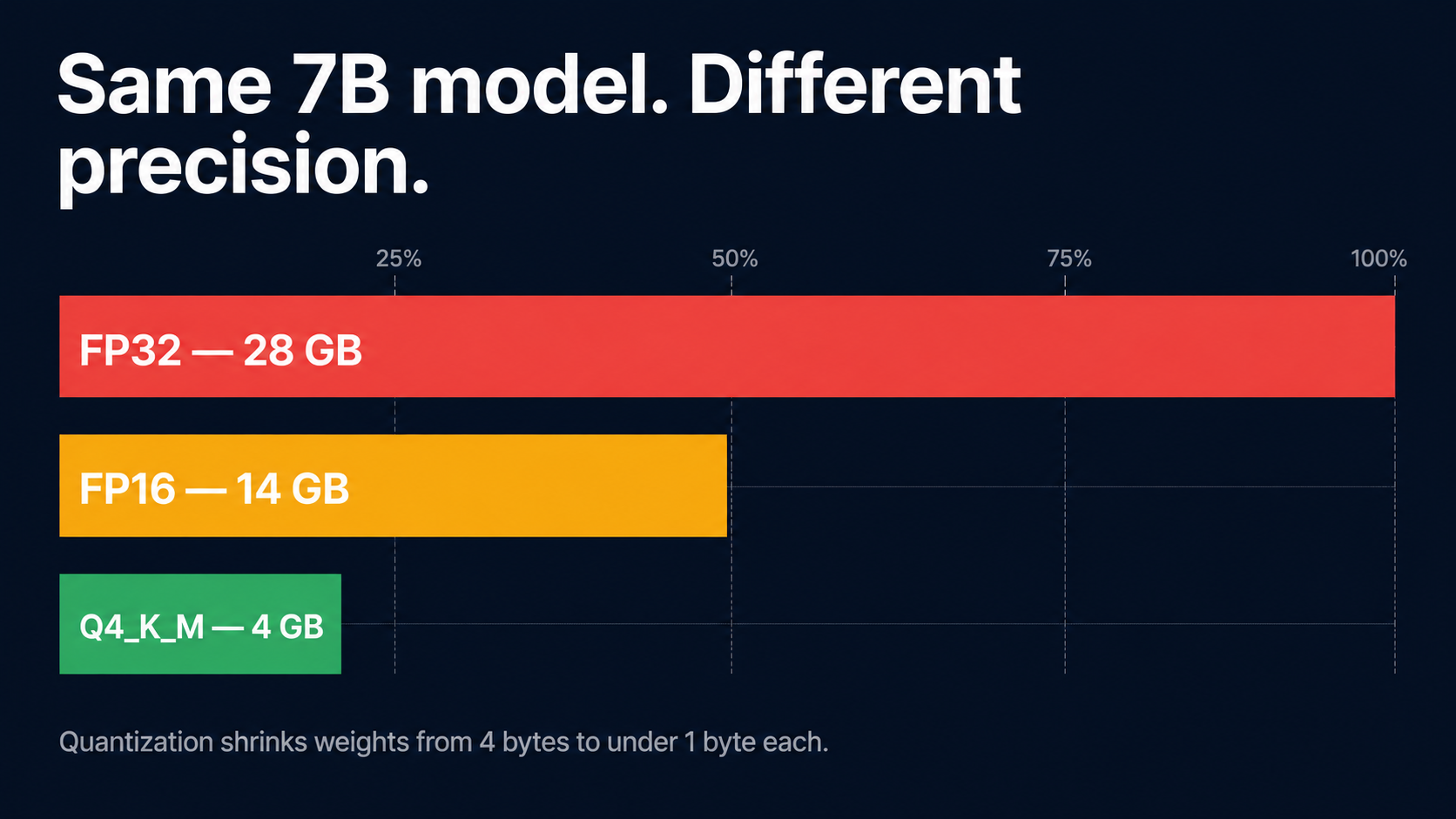
The same 7B model at three precisions. Quantization shrinks weights from 4 bytes to under 1 byte each.

1. Why we quantize at all

A modern LLM is, mechanically, a giant pile of numbers. A 7-billion-parameter model stored at full FP32 precision is 28 GB of weights — four bytes per parameter. A 70B model is 280 GB. The largest open models cross a terabyte. None of that fits in a consumer GPU. Even datacenter GPUs hit the wall fast.

Quantization is the trick that makes these models runnable on real hardware. The idea is simple: instead of storing each weight as a 32-bit (or 16-bit) float, store it using fewer bits — 8, 6, 5, 4, even 2 — and accept a tiny amount of error in return for a huge reduction in size and bandwidth.

• 28 GB — 7B model at FP32 (4 bytes per weight)
• 14 GB — same model at FP16 (2 bytes per weight)
• 4 GB — same model at Q4_K_M (~4.8 bits per weight)

The reason it works at all is that LLM weights are surprisingly tolerant of noise. They are billions of small numbers, mostly clustered near zero, and the network's output depends on a weighted sum across many of them. Small random errors mostly cancel.

But "4 bits" hides a lot of design choices. There are many different ways to spend those 4 bits — integer vs float, symmetric vs asymmetric, one scale per block of 32 vs scales stacked inside scales, importance-weighted vs uniform, stored vs natively computed. This post walks through each of them.

The single question that runs through the whole field: given a fixed bit budget per weight, where do you spend the bits? Every format on this page — Q4_K_M, IQ4_XS, MXFP8, NVFP4 — is a different answer to that one question. Keep that thread in mind; the rest is just variations on a theme.

2. Floats: what you're actually quantizing

Before quantization makes sense, you need to remember what a float is. Every floating point number has three parts:

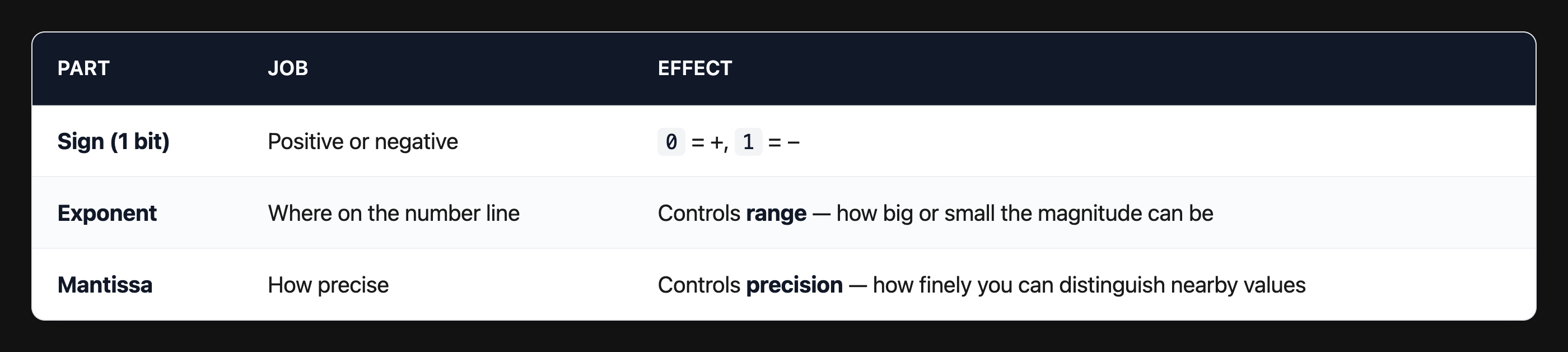
The shorthand EnMm means n exponent bits and m mantissa bits. So FP32 is E8M23, FP16 is E5M10, BF16 is E8M7 (same range as FP32 but less precision), FP8 (E4M3) is the most common 8-bit float, and FP4 (E2M1) is the new 4-bit one.

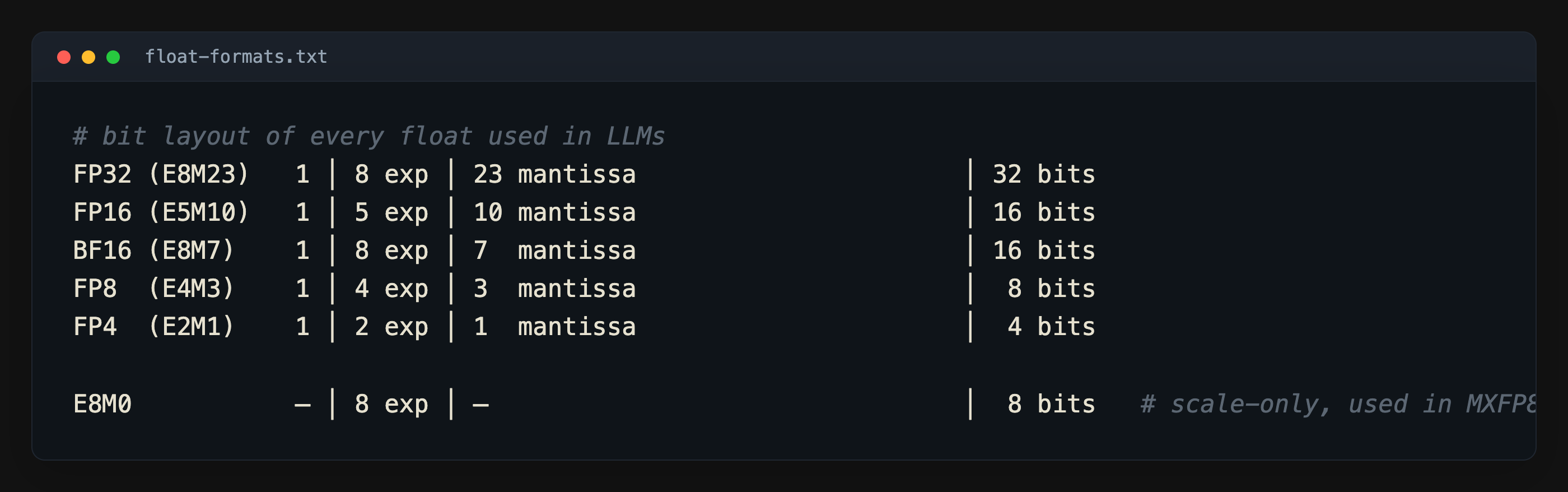
That last row, E8M0, is unusual: just an exponent, no sign, no mantissa. It can only represent powers of 2. It shows up later as the scale format in MXFP8.

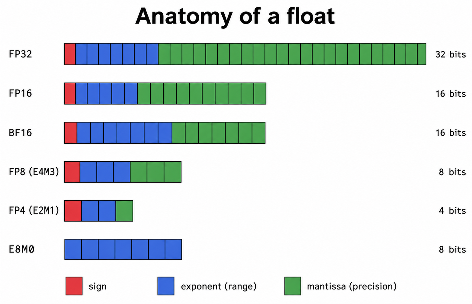
Every float is sign + exponent + mantissa. Each format splits the same bit budget differently.

One sentence to remember: exponent bits buy range, mantissa bits buy precision. Every format picks a different split of the same bit budget.

That range-vs-precision tradeoff is why BF16 dominates training while FP16 is mostly an inference format. Training gradients span 10+ orders of magnitude, and FP16's narrow 5-bit exponent overflows on the high end and underflows to zero on the low end. BF16's 8-bit exponent (same as FP32) handles the full range — at the cost of mantissa precision the optimizer doesn't really need.

🔗 Live version: drag a value and watch each format round it differently — gupta-bhavesh.github.io/visuals/float-anatomy

3. The core mechanic: block, slot, scale, dequantize

Every quantization scheme — old, new, integer, float — boils down to four ideas stacked on each other.

A weight is one number

A learned number inside the model. A 7B model has 7 billion of them. They live in matrices.

A block is a chunk of consecutive weights

You don't quantize each weight in isolation. You chop the flat weight array into blocks — usually 32 or 16 consecutive weights — and quantize each block as a unit. Block boundaries are purely sequential.

Why blocks at all? Because one scale for the entire layer would be too coarse — a single outlier weight would stretch the scale and waste precision for the other 16 million normal-sized weights.

A slot is one of the values your bits can represent

With N bits per weight, you have 2^N possible slots. At 4 bits that's 16 slots. At 2 bits that's 4 slots. At 8 bits that's 256.

The scale is the step size between slots

The scale is one float stored alongside each block that says: "to recover an approximate weight from a stored slot, multiply by this."

stored_int = round(original_float / scale)
recovered_float = stored_int × scale

The error between original and recovered is the quantization error. It's bounded by half a step — at most scale / 2 per weight.

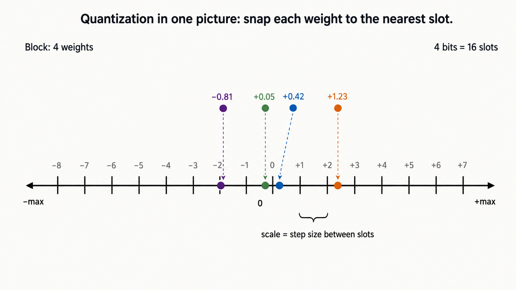
4-bit quantization in one picture: snap each weight to its nearest slot. Scale = the gap between slots.

A worked example

Suppose you have a block of 4 weights at 4-bit precision:

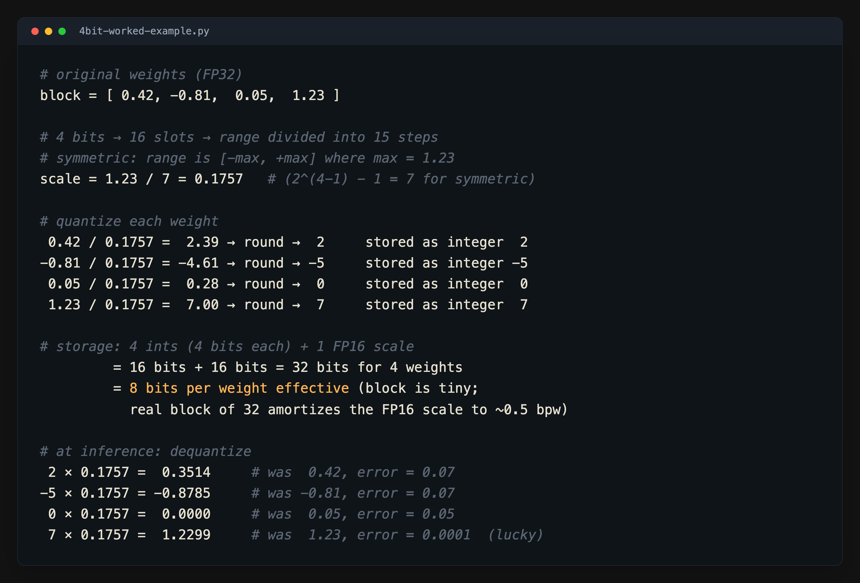
Every other format on this page — Q4_K_M, IQ4_XS, MXFP8, NVFP4 — is built from these same four ideas, just with different choices for slot spacing, block size, scale precision, and how the scales themselves are stored.

🔗 Live playground: drag a weight, change the bit depth, watch the error — gupta-bhavesh.github.io/visuals/quantization-playground

4. Symmetric vs asymmetric: do you need to store the min?

In symmetric quantization the formula is float = int × scale. Range is forced to [-max, +max]. Only the scale is stored — no "min."

In asymmetric quantization you store both a scale and a zero-point: float = (int − zero_point) × scale.

Trained model weights are almost always roughly zero-centered. Plot any layer's weights and you get a bell curve hugging zero. So symmetric wastes very little — both halves of the range are equally populated. Almost every weight quantization scheme is symmetric.

The exception is activations — values flowing between layers during inference. After a ReLU everything is ≥ 0, so a symmetric range would waste the entire negative half. Activations get asymmetric quantization. This matters when people quantize the KV cache at runtime — that's activation-derived state, and llama.cpp -ctv q4_1 uses asymmetric Q4_1 specifically because of it.

5. K-quants: scales stored inside scales

Storing a full FP16 scale for every 32 weights is wasteful — 16 bits of scale for 128 bits of weight data is a 12.5% overhead just on the scales. K-quants fix this by quantizing the scales themselves, then grouping multiple sub-blocks under one shared outer scale.

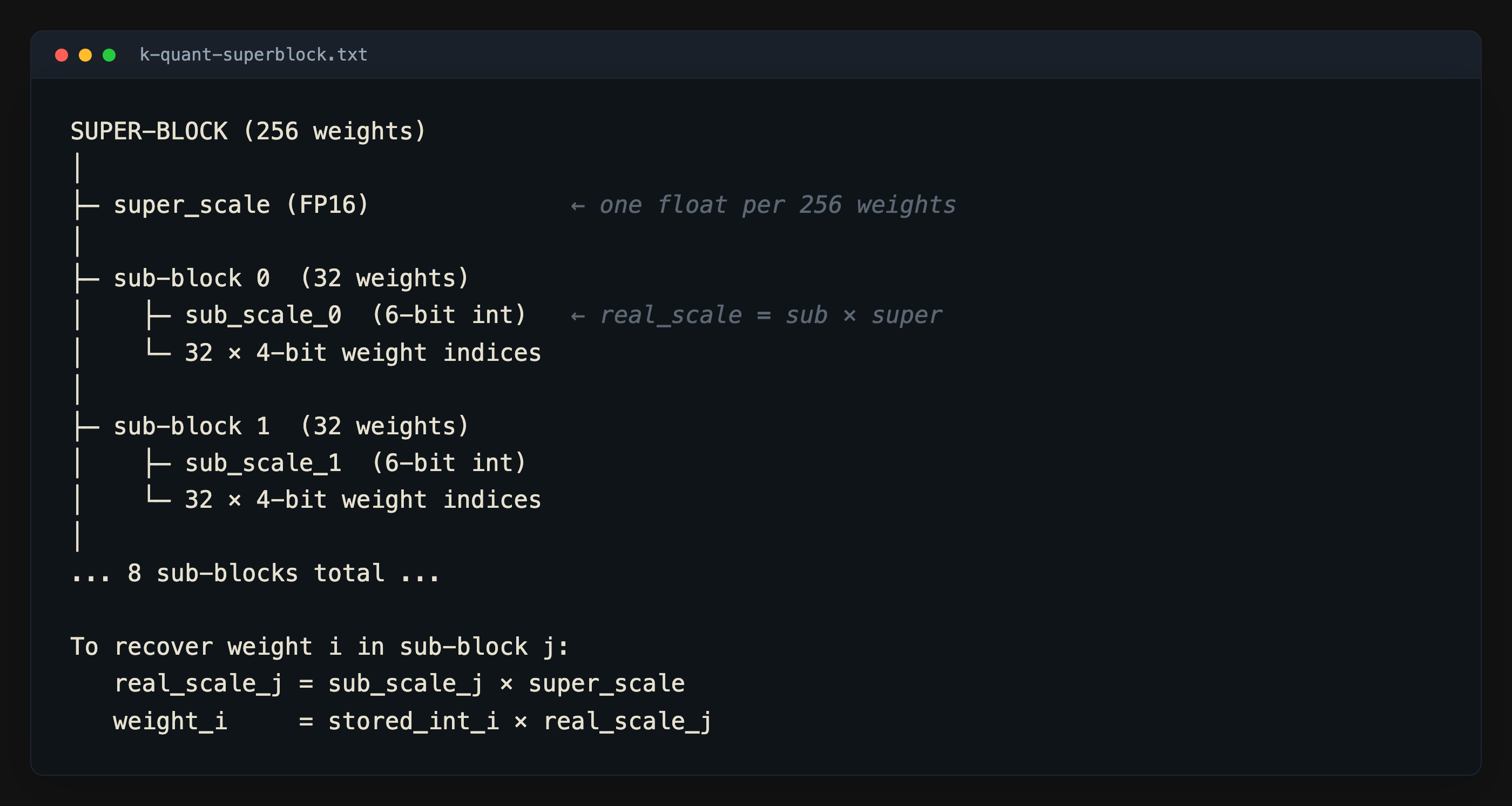
This hierarchy is the entire reason K-quants outperform legacy Q4_0 at similar bit depth. Two levels of scale give you per-sub-block precision while only paying for one FP16 number per 256 weights.

6. The GGUF zoo: every Q-format decoded

GGUF is the file format used by llama.cpp. Inside it, the quantization scheme for each tensor is one of about twenty named variants. The names look random at first — Q4_K_M, IQ3_XXS, IQ4_NL — but every piece of the name actually means something.

The naming grammar

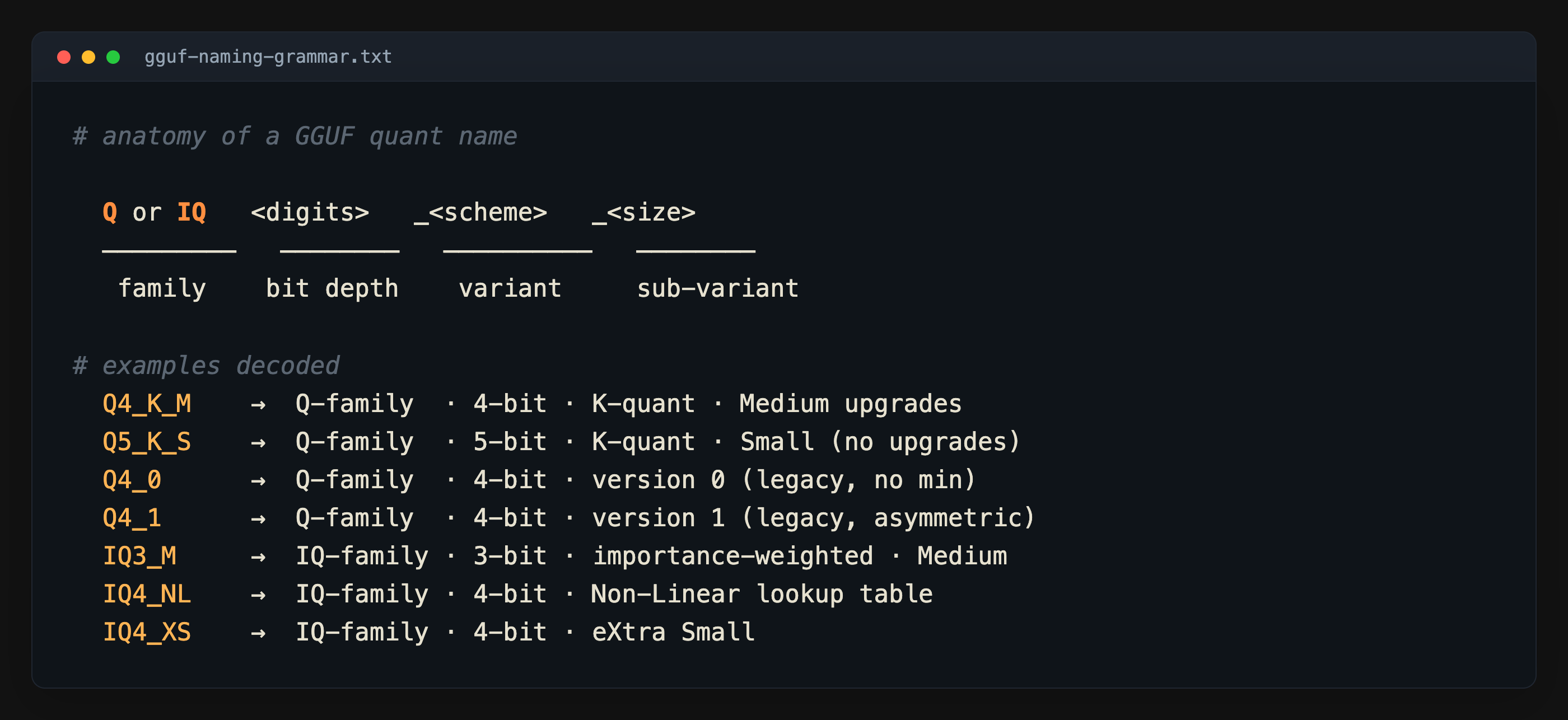
What each token means

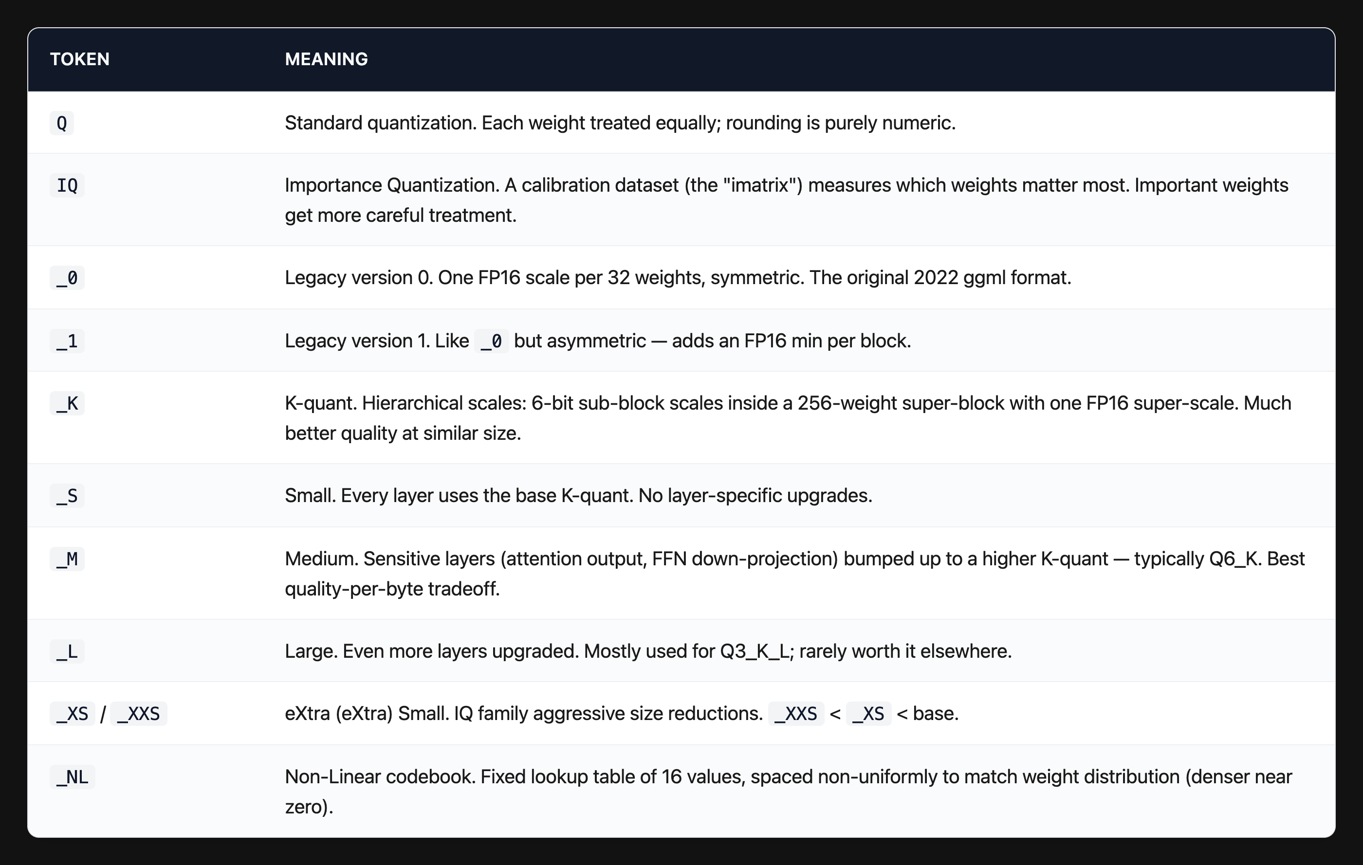
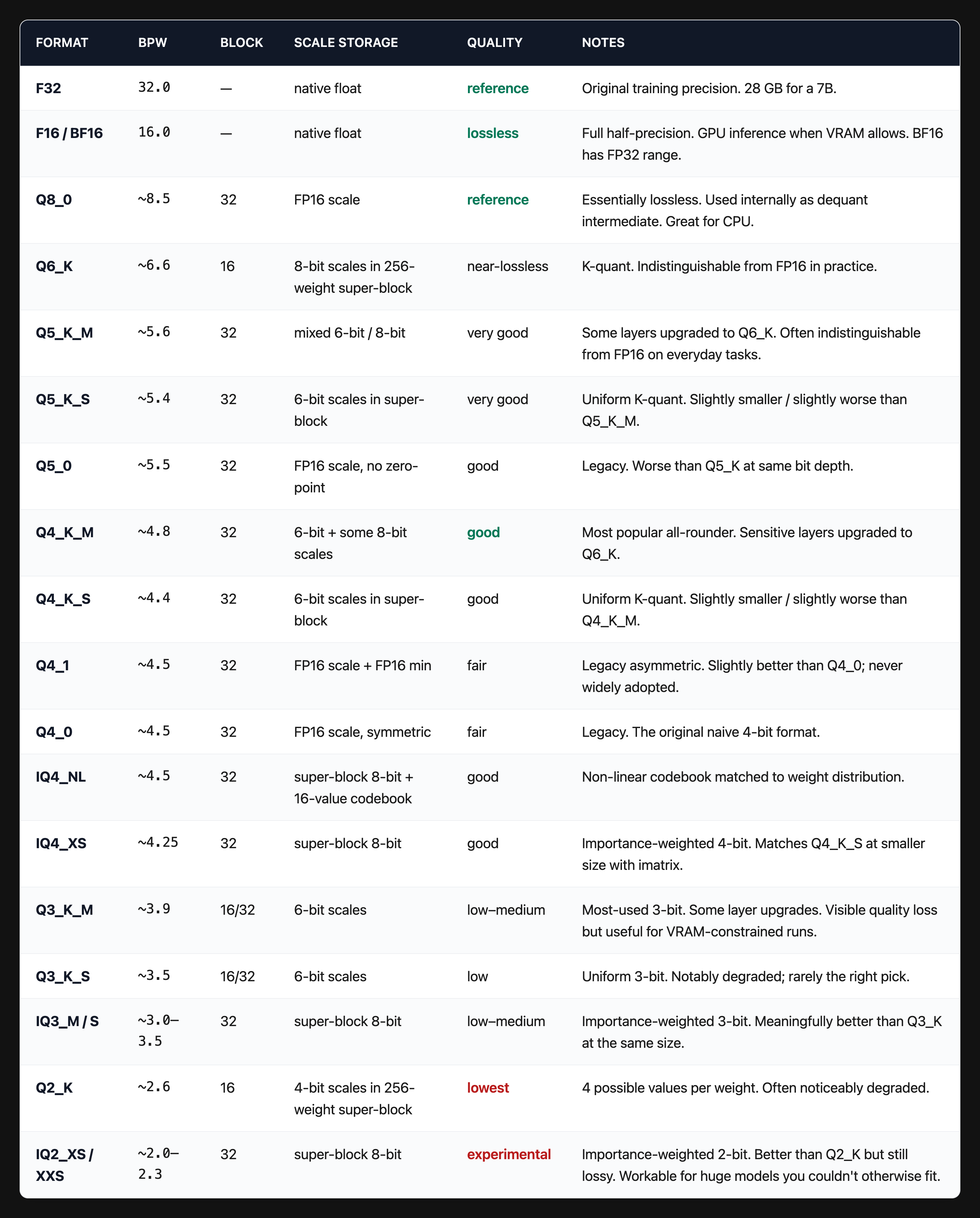
The full table

Quick read: lower bpw (bits per weight) means smaller file and more quality loss. Q4_K_M is the standard pick — everything else is a tradeoff against it.

Reading a real filename

llama-3-70B-Instruct-Q5_K_M.gguf:

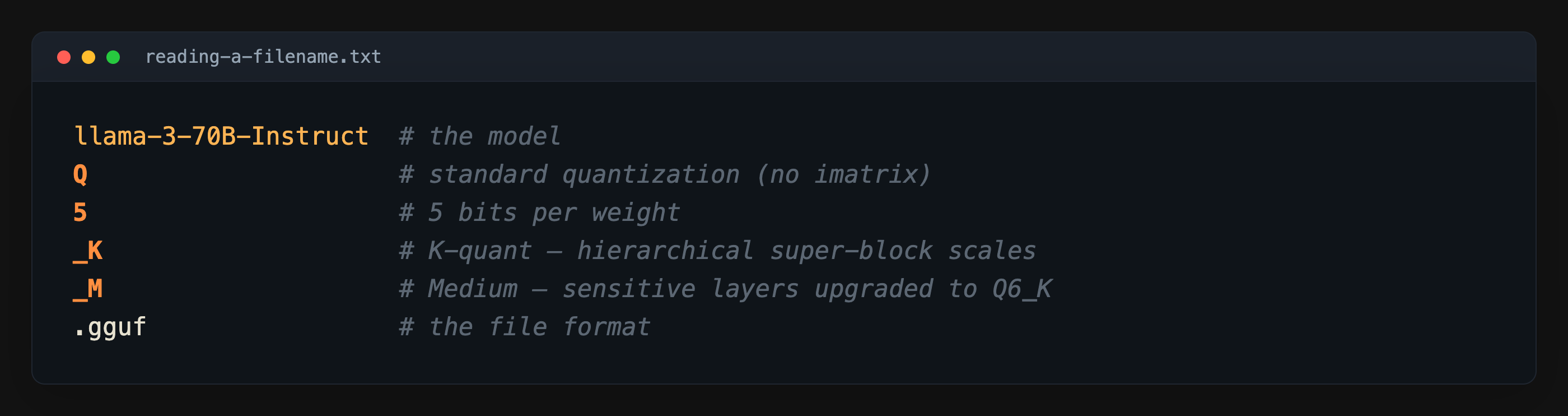
From the name alone you know: ~5.6 bpw effective, 32-weight blocks, 6-bit sub-block scales under FP16 super-scales, attention output and FFN down-proj layers run at Q6_K. Roughly 49 GB on disk for the full 70B.

7. IQ-quants: importance matrices

Standard Q-quants treat every weight identically. Each one gets snapped to its nearest slot purely on the basis of its numeric value. IQ-quants break that assumption.

The insight: not every weight matters equally to the model's output. Some weights, when perturbed by 0.01, change the final logits dramatically. Others can be perturbed by 0.1 with almost no measurable effect.

How importance is measured

Before quantization, you run a small calibration dataset (a few hundred chunks of text) through the model in FP16. For each weight, you measure how sensitive the output is to that weight. The result is an importance matrix (imatrix).

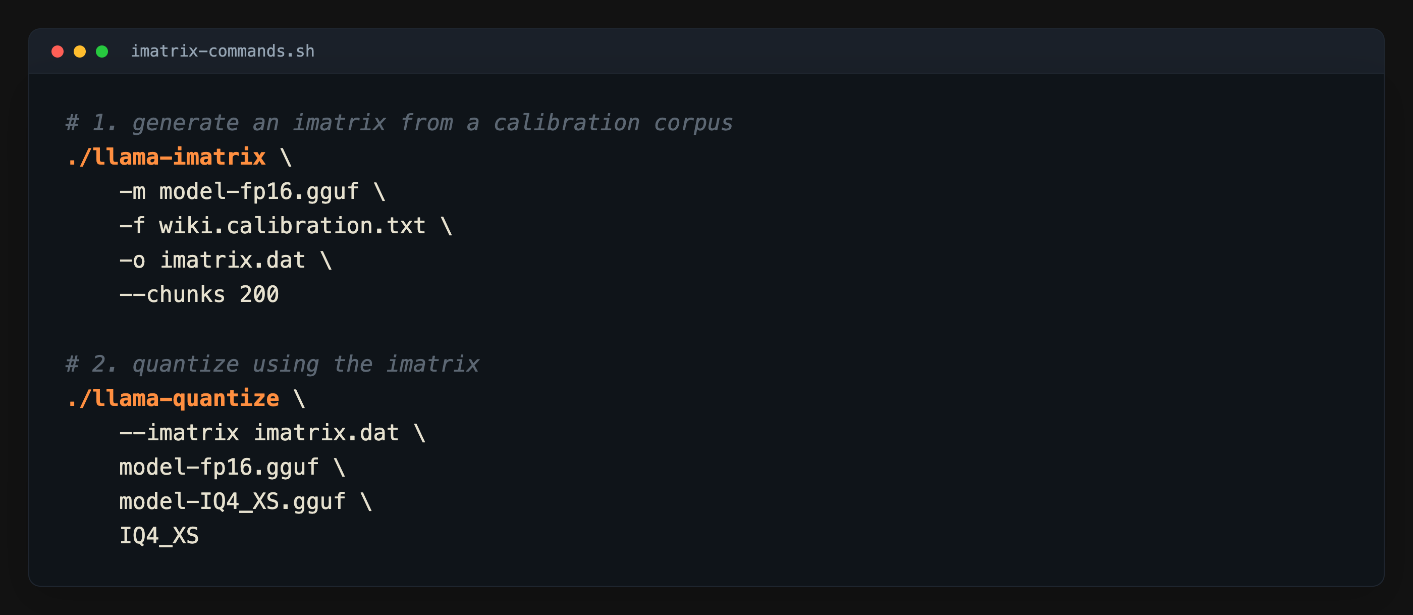
The non-linear codebook (NL)

IQ4_NL adds another twist on top: the slot positions themselves are not evenly spaced. Instead of dividing the range into 16 equal steps, IQ4_NL uses a fixed lookup table of 16 carefully chosen values, clustered more densely near zero (where most weights actually live).

This is the same idea as the NF4 format used by BitsAndBytes for QLoRA fine-tuning — slot positions placed at quantiles of a normal distribution.

8. Storage vs compute quantization

There's a critical distinction the older guides skip. It separates GGUF from MXFP8 and NVFP4.

Storage quantization (Q4_K_M, GPTQ, AWQ, EXL2): weights are stored compressed, but at inference time the runtime dequantizes them back to FP16 in registers before feeding into the tensor cores. The matrix multiply itself runs at FP16. You save memory and memory bandwidth — huge wins, since LLM inference is bandwidth-bound — but the actual arithmetic is unchanged.

Compute quantization (FP8, MXFP8, NVFP4): weights are stored compressed AND the tensor cores natively multiply in that reduced precision. No dequantize step. Faster on two axes: less data to move AND cheaper math per multiply. Requires hardware that physically supports the format.

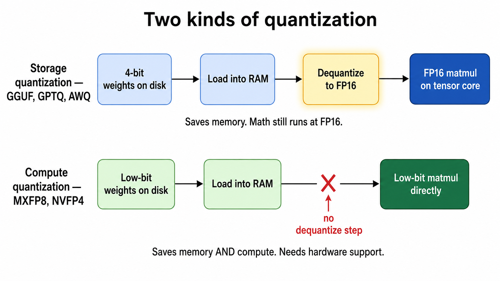
Storage quant saves memory only. Compute quant saves memory and compute — but needs hardware that natively does the low-precision math.

The lesson: GGUF saves you memory. MXFP8 / NVFP4 save you memory AND compute. But compute quantization is locked to whatever silicon happens to support that exact format — a hardware support problem more than a math problem.

Apple Silicon changes the calculation slightly. Unified memory means the CPU and GPU share one physical bandwidth pool — there's no separate VRAM to transfer weights into. Storage quantization wins are still real (less bandwidth consumed per matmul), but the "fit it in VRAM" framing doesn't apply. An M-series Mac can run a Q4_K_M 70B because the model just sits in regular RAM that the GPU can read directly, no copy step. CPU and GPU contend for that shared bandwidth, so quantization gains show up as throughput rather than as a binary fits/doesn't-fit.

9. MXFP8: microscaling FP8

MXFP8 is the format that finally took FP8 from "interesting research" to "production inference." It was standardized by AMD, Arm, Intel, Meta, Microsoft, Nvidia, and Qualcomm together through the Open Compute Project (OCP MX v1.0, September 2023) — so the same format runs natively on H100, MI300, Gaudi 3, and Blackwell.

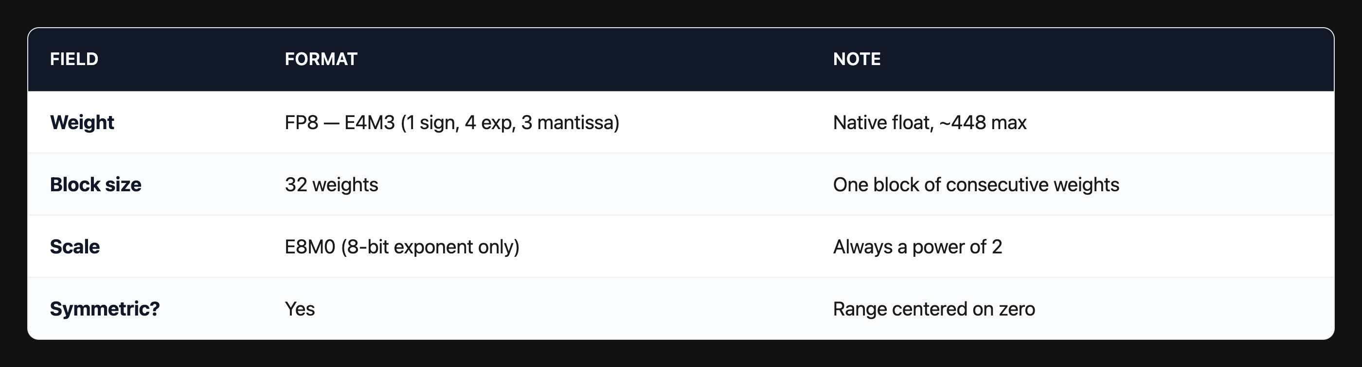
Why E8M0 for the scale?

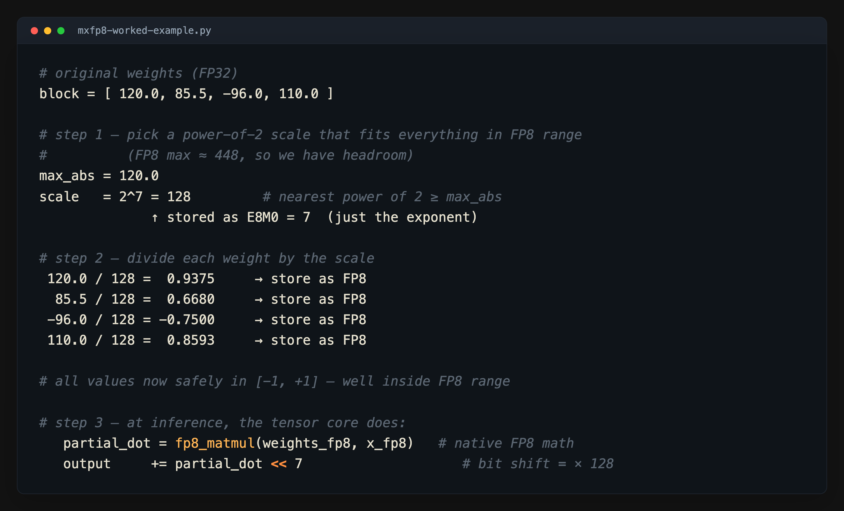
E8M0 has only 256 possible values — all powers of 2. That sounds restrictive, but it makes the hardware extremely fast: multiplying by a power of 2 is a bit shift, not a real float multiply. The tensor core can apply the scale to a partial dot-product result with just a shifter, costing essentially nothing.

A worked MXFP8 example

10. NVFP4: native 4-bit floats on Blackwell

NVFP4 is Nvidia's proprietary 4-bit float format, introduced with Blackwell (RTX 50, GB200).

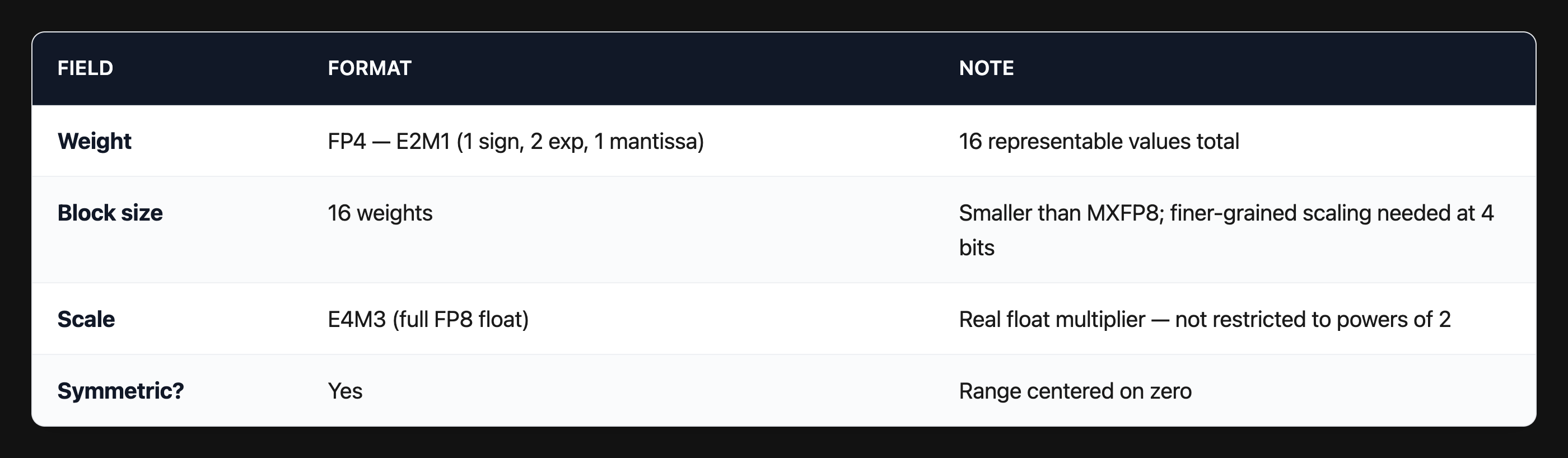
The 16 values of FP4 are not evenly spaced — the floating point format clusters them around small magnitudes: 0, ±0.5, ±1, ±1.5, ±2, ±3, ±4, ±6.

Why the scale is FP8, not E8M0

With only 16 slots to work with, getting the scale exactly right is critical. A power-of-2 scale would force the entire block to snap to whichever power of 2 is closest, potentially wasting half the precious slots. A full FP8 scale can be tuned freely.

A worked NVFP4 example

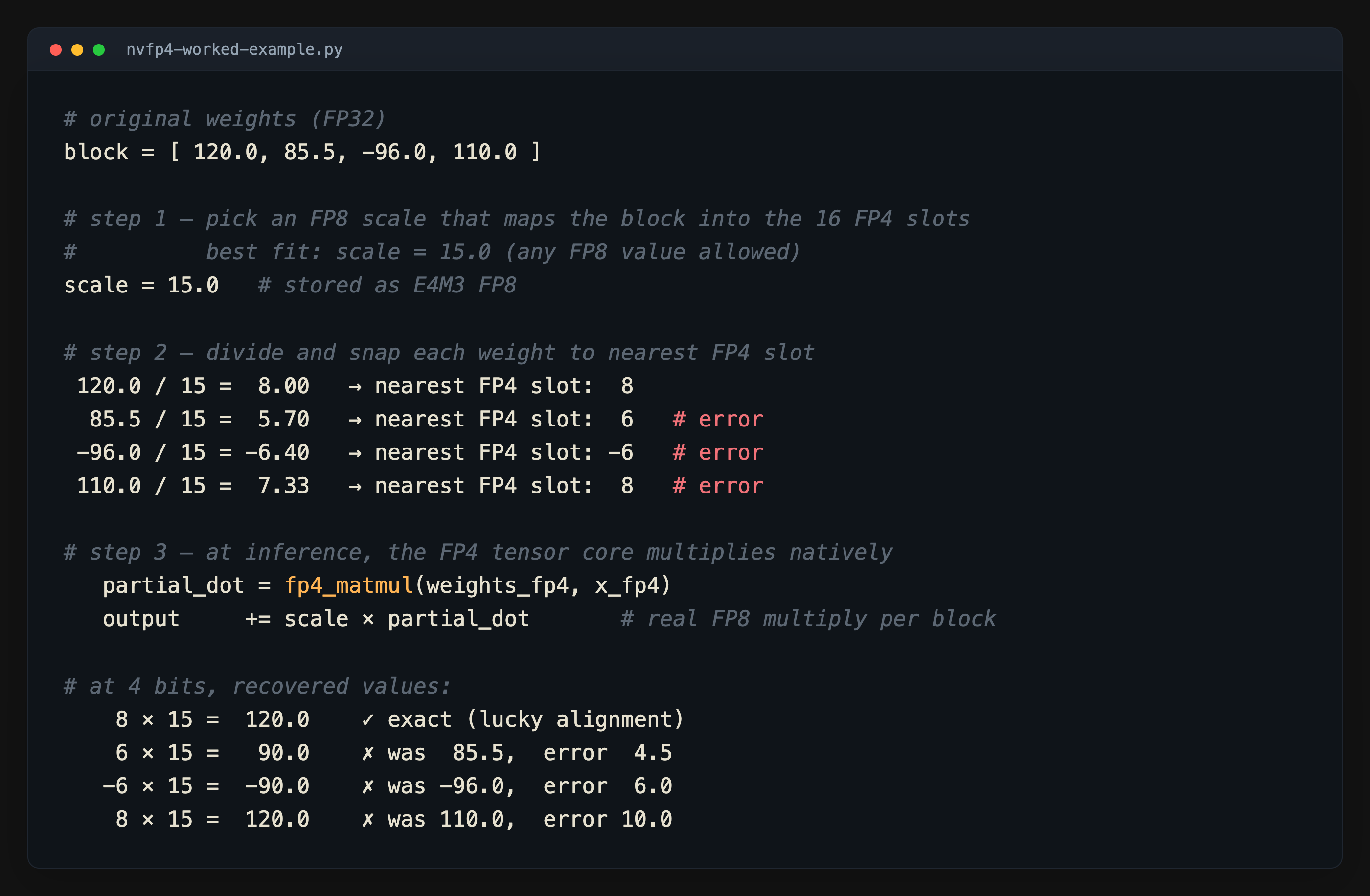
The scale multiply is not a single step at the end of the entire matrix multiply. It happens per block, interleaved into the accumulation. The 16:1 ratio of FP4 multiplies to scale applications is what keeps the whole thing fast.

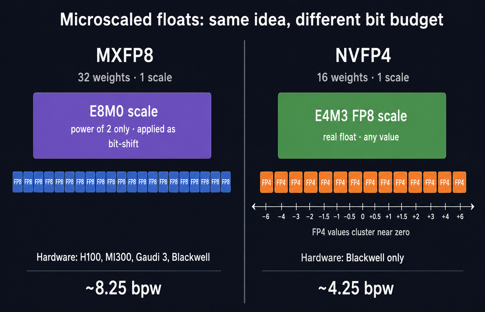
Same idea, different bit budget: MXFP8 has 32 FP8 weights and a cheap power-of-2 scale; NVFP4 has 16 FP4 weights and a real FP8 scale.

🔗 Live comparison: edit a block of weights and watch both formats round it — gupta-bhavesh.github.io/visuals/mx-vs-nv

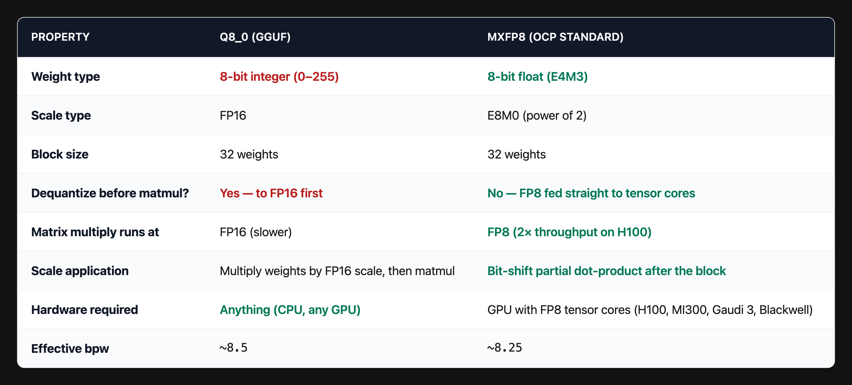
11. Q8_0 vs MXFP8: a direct side-by-side

Both formats are nominally "8-bit weights with one scale per 32." The difference is the entire reason MXFP8 is faster.

12. Why each format needs new silicon

A natural question: if a GPU can do FP8 math, why can't it do FP4?

A tensor core is a small piece of silicon hardwired to do exactly one operation: multiply two matrices of a specific format and accumulate the result. It's not flexible software — it's physical circuits etched into the chip, sized for specific bit widths and specific exponent/mantissa splits.

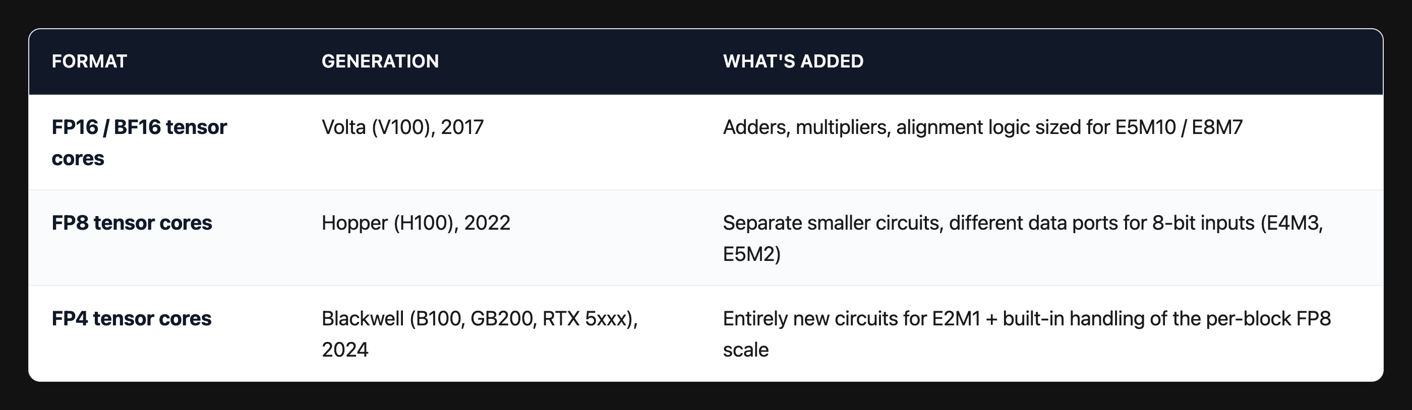
FP8 hardware cannot ingest 4-bit inputs at all — its data ports literally expect 8-bit values. Each new format requires new silicon. Each generation Nvidia adds tensor core blocks to the chip — the FP16 tensor cores from Volta are still in Blackwell, just sitting alongside newer FP8 and FP4 cores.

13. Beyond GGUF: GPTQ, AWQ, EXL2, NF4

llama.cpp's GGUF formats are designed for portability. The other major quantization families take different design tradeoffs, mostly aimed at GPU-only inference or fine-tuning.

GPTQ uses second-order information (the Hessian of the loss) during quantization. Round one weight, measure the error, compensate by adjusting nearby weights before rounding them. Errors propagate in a controlled chain. GPU only.

AWQ noticed that weights multiplied by large activations matter more — their rounding errors get amplified. So AWQ scales those weights up before quantizing them, then scales the activations down to cancel it out.

EXL2 lets you set a target average bpw (say 4.5) — the quantizer figures out which layers can tolerate 3-bit and which need 5-bit. Most flexible GPU format.

BitsAndBytes / NF4 is "NormalFloat 4-bit" — slot positions placed at quantiles of a standard normal distribution. Primarily a training format for QLoRA fine-tuning.

14. Where in the model: what gets quantized

"Quantize the model" is a simplification. A transformer has many tensor types and they're not equally tolerant of low-precision storage.

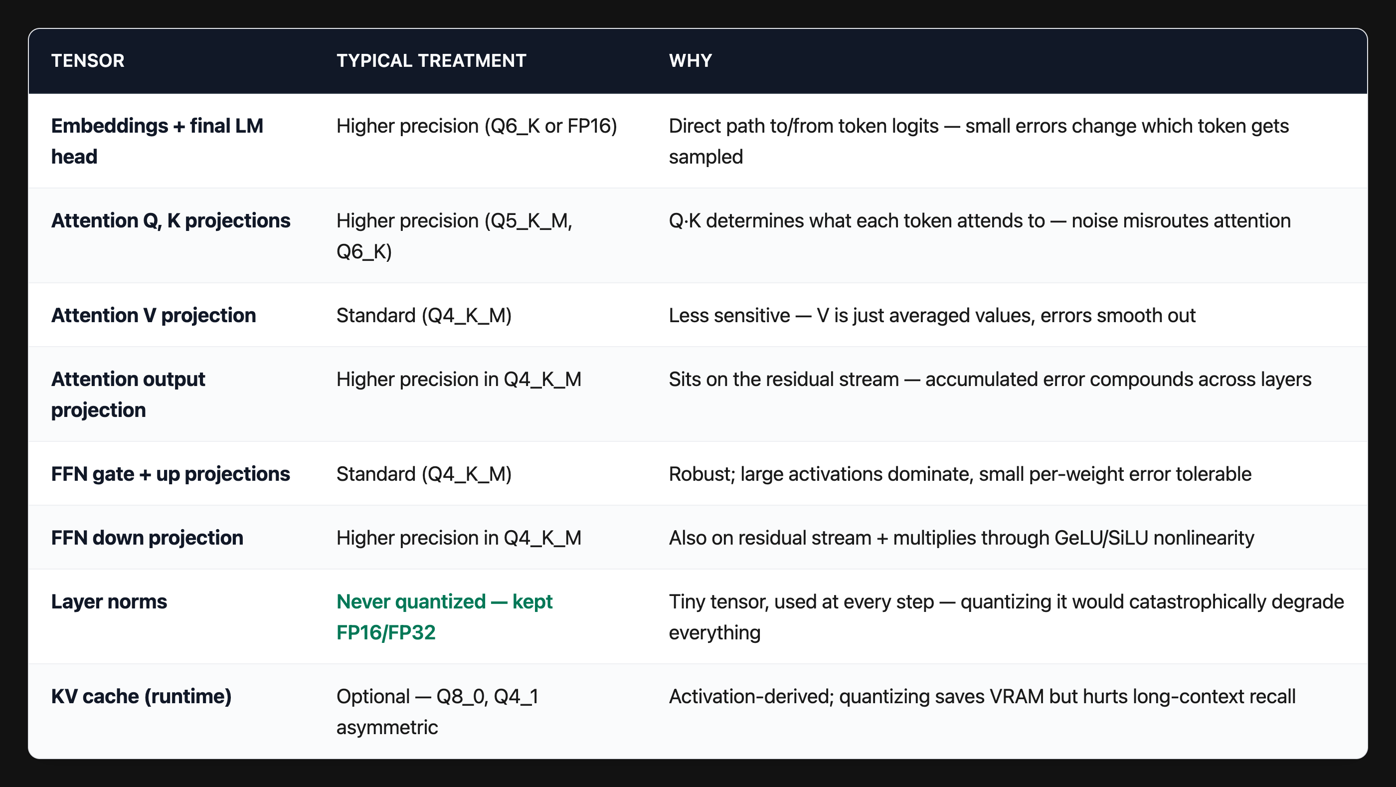
The "_M" in K-quants exists exactly to encode this layer-by-layer policy.

15. llama.cpp: the commands that actually do it

If you just want to download a pre-quantized model from Hugging Face, skip this section. The commands below are for converting and quantizing a model yourself with llama.cpp.

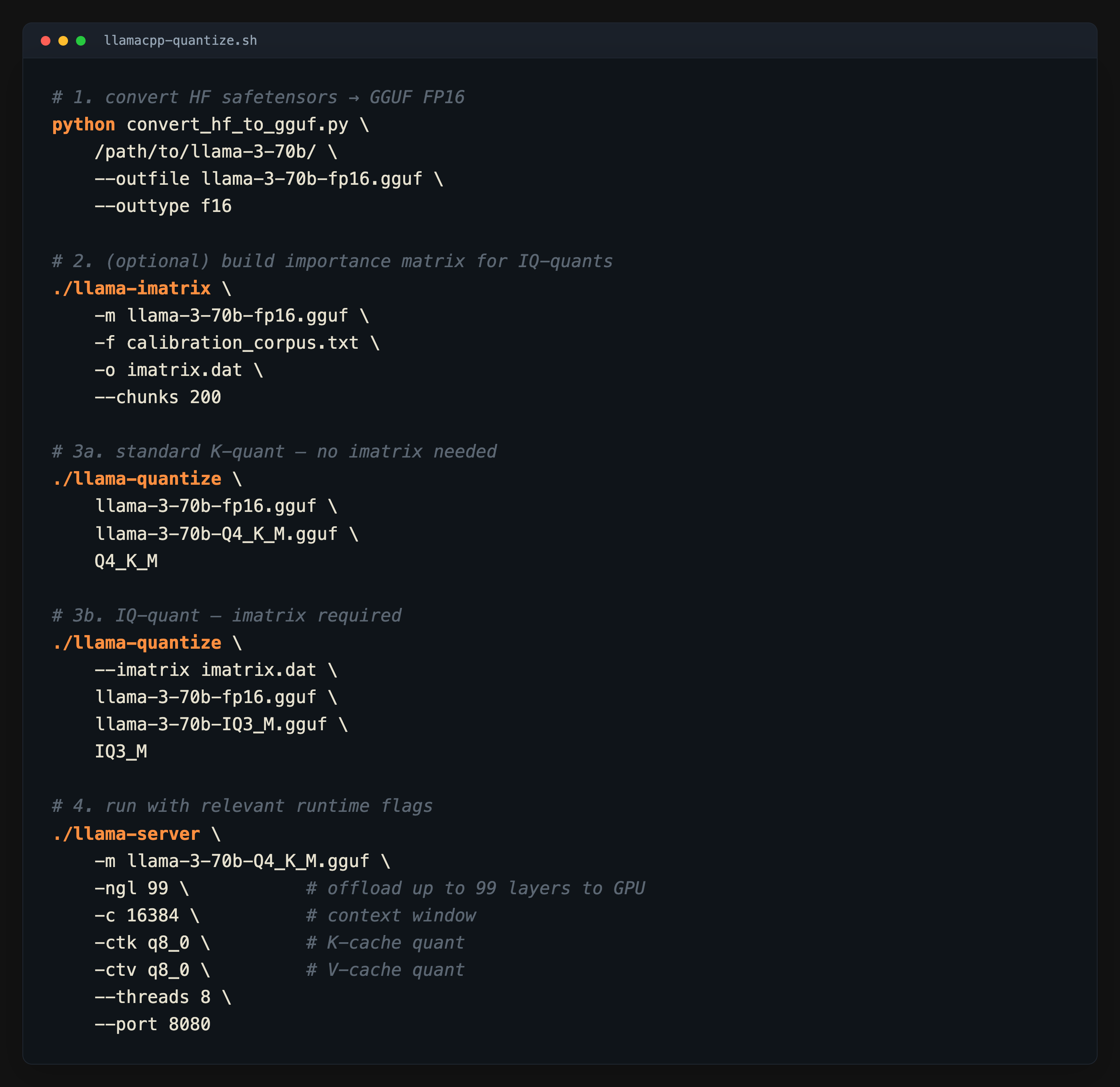
-ngl controls CPU/GPU split. With -ngl 0 everything runs on CPU; with -ngl 99 the entire model goes to GPU if it fits. Partial offload — say -ngl 32 on a 60-layer model — runs the bottom 32 layers on GPU and the rest on CPU.

16. Choosing: which quant should you pick?

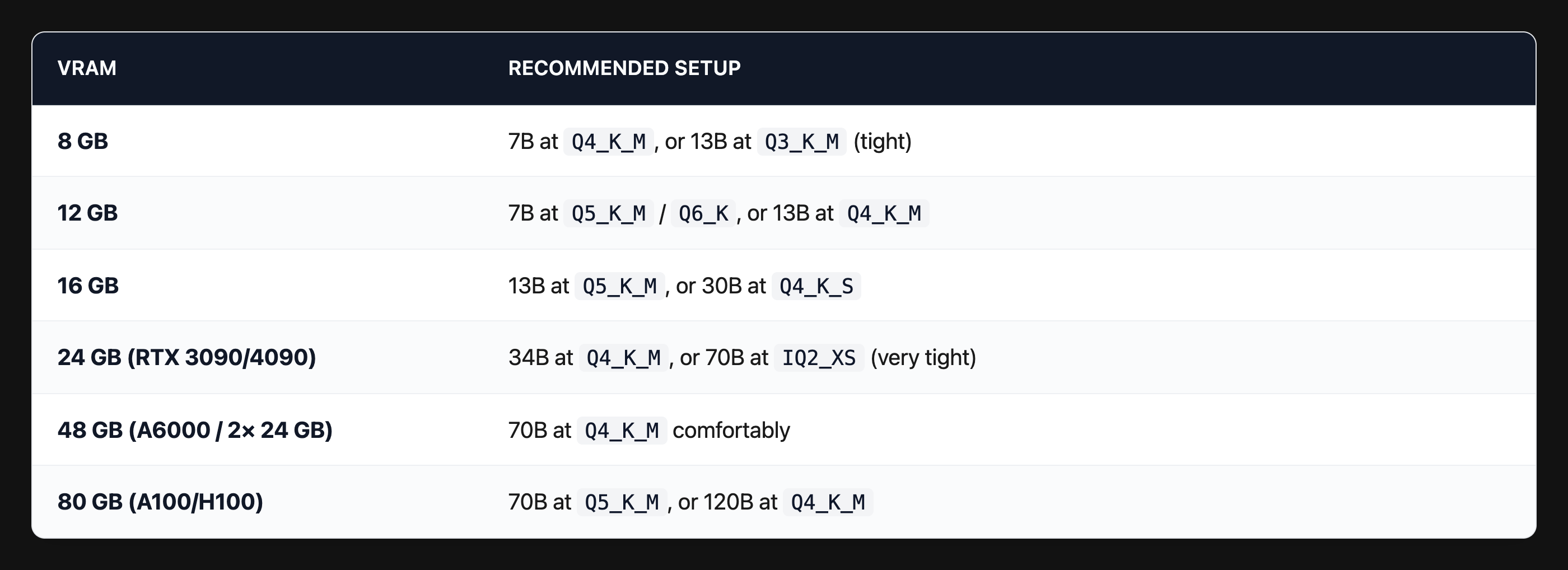
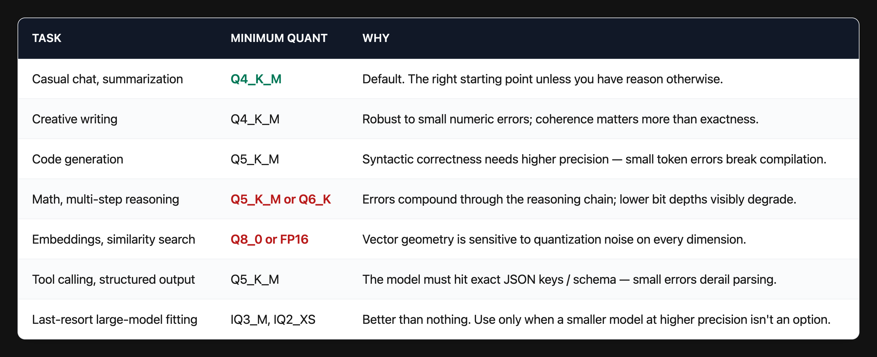
The default: Q4_K_M is the safe default. Go lower only when forced by VRAM. Go higher when doing precision-sensitive work.

17. The bigger picture

Every quantization scheme on this page is a different answer to the same question: given a fixed bit budget per weight, where do you spend the bits?

Legacy formats (Q4_0) spent them naively: one FP16 scale per block, evenly spaced slots, every weight treated equally. K-quants spent some bits on a hierarchy of scales. IQ-quants spent some on importance metadata. Non-linear codebooks spent some on slot positions matched to the actual weight distribution. MXFP8 and NVFP4 spent some on having a real float representation that the hardware can compute on directly. Each generation has been a slightly more sophisticated answer to "where does precision actually matter?"

The pattern that runs through all of them is the same four-line recipe: chop weights into blocks, find a scale per block, snap each weight to the nearest available slot, store the slot and the scale.

The takeaway: quantization is not magic and it's not lossy compression in the JPEG sense. It's the deliberate trading of per-weight precision for total bandwidth, made survivable by the fact that LLM outputs depend on millions of weighted sums where random errors cancel. Once the block/scale/slot pattern clicks, every cryptic filename tells you exactly what's inside.